Line Optimization in Public Transport
The line optimization problem in public transport is to choose a set of lines (routes in the transportation network) with associated frequencies (how often the lines are operated) such that a given transportation demand can be satisfied. This problem is an example of a classical network design problem. There are different approaches and models to solve the line optimization problem. A general overview on models and methods is given by Schoebel [1].
For this optimod we assume we are given a public transportation network, being a set of stations and the direct links between them. We are given the origin-destination (OD) demand, i.e., it is known how many passengers want to travel from one station to another in the network within a considered time horizon. We are also given a set of possible lines. A line is a path a public transportation network. We call a subset of these lines where each line is associated with a frequency a line plan. The optimod computes a line plan with minimum cost such that the capacity of the chosen lines sufficient to transport all passengers.
We provide two different strategies to find a line plan with minimum cost:
The first approach assumes that passengers only travel from their origin to their destination along the path with the shortest travel time. For this purpose, all shortest paths are computed for each OD pair and it is only allowed to route passengers along these paths.
The second approach does not restrict the passenger paths, but instead applies a multi-objective approach. In the first objective the cost of the line plan is minimized such that all passenger demand can be satisfied. In the second objective the travel time for the passengers is minimized such that the cost of the line plan increases by at most 20% over the minimum cost line plan.
Problem Specification
Let a graph \(G=(V,E)\) represent the transportation network. The set of vertices \(V\) represent the stations and the set of edges \(E\) represent all possibilities to travel from one station to another without an intermediate station. A directed edge \((u,v)\in E\) has the attribute time \(\tau_{uv}\geq 0\) that represents the amount of time needed traveling from \(u\) to \(v\). For each pair of nodes \(u,v\in V\) a demand \(d_{uv}\geq 0\) can be defined. The demand represents the number of passengers that want to travel from \(u\) to \(v\) in the considered time horizon. Let \(D\) be the set of all node pairs with positive demand. This set is also called OD pairs. Further given is a set of lines \(L\). A line \(l\in L\) contains the stations it traverses in the given order. If a line runs in both directions, it needs to be repeated in reverse order.
A line has the following additional attributes:
fixed cost: \(C_{l}\geq 0\) for installing the line
operating cost: \(c_{l}\geq 0\) for operating the line once in the given time horizon
capacity: \(\kappa_{l}\geq 0\) when operating the line \(l\) once in the given time horizon
Additionally, we have a given list of frequencies. The frequencies define the possible number of operations for the lines in the given time horizon. If a line \(l\) is operated with frequency \(f\) the overall cost for the line is \(C_{lf}=C_l + c_{lf}\cdot f\) and the total capacity provided by the line is \(\kappa_{l,f}=\kappa_l\cdot f\).
The problem can be stated as finding a subset of lines and associated frequencies with minimal total cost such that all passengers can be transported.
Background: Optimization Model with Approach 1
In an initial step the all-shortest-paths algorithm of networkx is used to compute all travel time shortest paths for each OD pair. Let \(P_{st}\) be the set of all such shortest paths for OD pair \((s,t)\). Then variables \(y^{st}_{p}\) are defined for each path \(p\in P_{st}\). We have binary variables \(x_{l,f}\) for each line frequency combination indicating if line \(l\) is operated with frequency \(f\).
This Mod is implemented by formulating a Linear Program (LP) and solving it using Gurobi. The formulation can be stated as follows:
The objective minimizes the total cost of a line plan. The first constraint ensures that a line is associated with at most one frequency. The second constraint ensures that the line capacities can serve the passenger routing on shortest paths. The third constraint requires that the demand is routed on the precomputed shortest paths. The last two constraints ensure non-negativity of the variables and the line-frequency variables to be binary.
Background: Optimization Model with Approach 2
This Mod is implemented by formulating a Linear Program (LP) and solving it using Gurobi. We have binary variables \(x_{l,f}\) for each line frequency combination indicating if line \(l\) is operated with frequency \(f\). We define continuous variables \(y_{suv}\geq 0\) for the number of passengers starting their trip in station \(s\) and traveling on edge \((u,v)\).
The formulation can be stated as follows:
The objective minimizes the total cost for the chosen lines in a first objective and minimizes the total travel times for all passengers in the second objective.
The first constraint ensures that a line is associated with at most one frequency. The second constraint ensures that the line capacities can serve the passenger routing. The third and fourth constraints define a passenger flow for the given demands.
The last two constraints ensure non-negativity of the variables and the line-frequency variables to be binary.
Code and Inputs
This Mod can be used with pandas using a pd.DataFrame.
An example of the inputs with the respective requirements is shown below.
>>> from gurobi_optimods import datasets
>>> node_data, edge_data, line_data, linepath_data, demand_data = datasets.load_siouxfalls_network_data()
>>> node_data.head(4)
  number      posx      posy
  0   1       50000.0   510000.0
  1   2       320000.0  510000.0
  2   3       50000.0   440000.0
  3   4       130000.0  440000.0
>>> edge_data.head(4)
      source  target  length  time
  0   1       2       0.010   360
  1   2       1       0.010   360
  2   1       3       0.006   240
  3   3       1       0.006   240
>>> line_data.head(4)
  linename    capacity        fix_cost        operating_cost
  0   new7_B  600     15      3
  1   new15_B 600     15      2
  2   new23_B 600     15      6
  3   new31_B 600     15      6
>>> linepath_data.head(4)
  linename    edge_source     edge_target
  0   new7_B  1       2
  1   new7_B  2       6
  2   new7_B  6       8
  3   new7_B  8       6
>>> demand_data.head(4)
  source      target  demand
  0   1       2       5
  1   1       3       5
  2   1       4       25
  3   1       5       10
>>> frequencies = [1,3]
For the example we used data of the Sioux-Falls network. It is not considered as a realistic one. However,
this network can be found on different websites when considering traffic problems
(originally by Hillel Bar-Gera http://www.bgu.ac.il/~bargera/tntp/). We added a set of line routes.
Note that the output shown above contains some additional information that is not required for computation, for example
the property length in the edge data.
Also, posx and posy in the node_data is not used for computation. But it can be used to visualize the
network as done below.
It is important that all data is consistant. For example, edge_source, edge_target
in the linepath_data must correspond to a number in the node_data. The same holds
for source and target in edge_data and demand_data.
In the code it is checked that all tables provide the relevant columns.
Note that the edges are assumed to be directed and both direction need to be defined if an edge
can be traversed in both directions. In the same way, a line is a directed path. If a line is
turning at the end point and goes back the same way, the nodes need to be added again in reverse order.
Solution
The solution consists of two information
the total cost of the optimal line plan
the optimal line plan as a list of linename-frequency tuples.
The strategy can be defined via a Boolean parameter shortestPaths. This parameter has a default value (True) which uses approach 1, i.e., routing passengers on shortest paths only. Note that strategy 1 needs the python package networkx. If this is not available, the second approach is used. The second approach is also used if the parameter shortestPaths is set to False.
>>> from gurobi_optimods import datasets
>>> from gurobi_optimods.line_optimization import line_optimization
>>> node_data, edge_data, line_data, linepath_data, demand_data = datasets.load_siouxfalls_network_data()
>>> frequencies = [1,3]
>>> obj_cost, final_lines = line_optimization(node_data, edge_data, line_data, linepath_data, demand_data, frequencies, True, verbose=False)
>>> obj_cost
211.0
>>> final_lines
[('new271_B', 1), ('new31_B', 1), ('new407_B', 1), ('new415_B', 3), ('new423_B', 3), ('new535_B', 3), ('new551_B', 3), ('new71_B', 1)]
We provide a basic method to plot a line plan that has at most 20 lines using networkx and matplotlib. In order to use this functionality, it is necessary to install both packages if not already available as follows:
pip install matplotlib
pip install networkx
Additionally, the node_data must include coordinates for the node positions, i.e., the columns posx and posy
must be available. The plot function generates a matplot that is opened in a browser:
from gurobi_optimods.line_optimization import plot_lineplan
plot_lineplan(node_data, edge_data, linepath_data, final_lines)
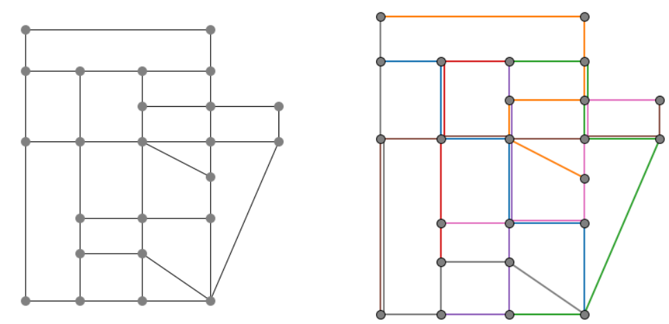
The Sioux-Falls transportation network (left) and the optimal line plan (right) for this example is shown in the figure below. The lines are shown as different colored paths in the network.