Bottleneck Hamiltonian Cycle
A Hamiltonian cycle visits every node of a graph exactly once before returning to where it started. When the arcs carry weights, a natural question is which Hamiltonian cycle has the smallest largest arc. This is the bottleneck (or min-max) Hamiltonian cycle problem, also known as the bottleneck traveling salesman problem (Garfinkel and Gilbert[1]).
Note that this is not the classical traveling salesman problem, which minimizes the total weight of the tour. Minimizing the largest arc and minimizing the sum of the arcs generally select different cycles, and the two answer quite different questions.
There are two useful ways to read the weights.
Weights as distances. Minimizing the longest single leg of a tour answers the question “what is the smallest range a vehicle needs in order to visit every location and come home?”. A tour is feasible for a vehicle exactly when its longest leg is within range, so the bottleneck of the best cycle is the minimum range that makes the trip possible at all.
Weights as availability times. If the weight of an arc is the moment that arc comes into existence, then a cycle only exists once all of its arcs exist, which is the moment its latest arc appears. Minimizing the maximum therefore answers “how early can a cycle be completed?”. The example on this page is of the second kind.
Problem Specification
Consider a directed graph \(G = (V, A)\) with \(n = |V| \geq 3\) nodes, where each arc \((i, j) \in A\) has a weight \(w_{ij}\). Find a directed Hamiltonian cycle \(C\) — a closed walk entering and leaving every node exactly once — which minimizes
Note that the weight values are not important — only their relative ordering. Any strictly increasing transformation of every weight leaves the optimal cycle unchanged, since it cannot alter which arc of a cycle is the largest. This is why dates, round numbers and distances are all equally valid inputs.
Background: Optimization Model
This Mod is implemented by formulating a Mixed Integer Programming (MIP) model and solving it using Gurobi. For each arc \((i, j) \in A\), define a binary decision variable
and let \(z\) be the largest weight used by the cycle. The model is
The first two constraints require every node to be left exactly once and entered exactly once. On their own they permit a solution to fall apart into several disjoint cycles, so the third family, the subtour elimination constraints of Dantzig et al.[2], forbids any proper subset of the nodes from closing a cycle among themselves. There are exponentially many of these, so the Mod adds them lazily: it solves without them and, whenever a candidate solution turns out to be several disjoint cycles, cuts each one off and continues. The compact formulation of Miller et al.[3] avoids the callback at the cost of a considerably weaker relaxation.
The constraint \(z \geq w_{ij} x_{ij}\) makes \(z\) at least as large as every arc the cycle actually uses, and since \(z\) is minimized it settles exactly on the largest of them.
Two refinements are worth mentioning, both used by the implementation. Because only the ordering of the weights matters, the model is built on the ranks of the distinct weight values rather than the values themselves, which keeps the objective integral and small and lets dates be used directly. And since every node must use one of its outgoing arcs and one of its incoming arcs, the bound
is valid and free to compute. It is often surprisingly strong; in the example below it is exactly the optimal value.
Background: when does a Hamiltonian cycle exist?
Deciding whether a directed graph contains a Hamiltonian cycle at all is NP-complete, which is why an optimization solver is a reasonable tool here even before any weights are involved.
There is a classical special case worth knowing. A tournament is a directed graph in which every pair of nodes is joined by exactly one arc, that is, a complete undirected graph with an orientation chosen for each edge. And a directed graph is strongly connected when every node can be reached from every other by following arcs.
Camion[4] showed that every strongly connected tournament contains a Hamiltonian cycle. Strong connectivity is necessary in any directed graph, since a Hamiltonian cycle itself reaches everything from everywhere, and for a tournament it is also sufficient. A linear-time check therefore decides the question outright: if the graph is strongly connected a cycle exists, and if it is not, for instance because some node has no outgoing arc, no cycle can exist. That is a strong statement about tournaments specifically, since strong connectivity is far from sufficient in general.
Coverage is what earns that conclusion, not uniqueness. The argument needs only that every pair of nodes be joined by at least one arc, so it survives unchanged when some pairs are joined in both directions; extra arcs cannot destroy a cycle. A pair joined by no arc is another matter, and then the graph really does fall outside the class and existence is a genuine question again. Knowing that some cycle exists says nothing about which one is best in any case.
One necessary condition is checked before the model is built: every node
needs at least one incoming and one outgoing arc. If some node has neither,
the Mod raises a ValueError naming it, rather than reporting an
unhelpful infeasible model.
Interface
The min_bottleneck_hamiltonian_cycle function accepts a scipy sparse array,
a networkx graph, or a pandas dataframe. Weights are optional in all three
cases and default to one, in which case the Mod simply returns some Hamiltonian
cycle if one exists.
The graph is a dataframe indexed by ("source", "target") with a
weight column. Columns of those names are accepted too.
>>> import pandas as pd
>>> from gurobi_optimods.hamiltonian_cycle import min_bottleneck_hamiltonian_cycle
>>> arcs = pd.DataFrame(
...     [("a", "b", 1), ("b", "c", 6), ("c", "d", 2), ("d", "a", 3),
...      ("a", "c", 4), ("c", "b", 3), ("b", "d", 5)],
...     columns=["source", "target", "weight"],
... ).set_index(["source", "target"])
>>> min_bottleneck_hamiltonian_cycle(arcs, verbose=False)
HamiltonianCycleResult(cycle=['a', 'c', 'b', 'd'], weights=[4, 3, 5, 3], bottleneck=5)
The graph is a square sparse array whose stored entries are the arc
weights. Note that a stored zero is a genuine arc of weight zero, so
take care not to let it be dropped, for example by
eliminate_zeros().
>>> import numpy as np
>>> import scipy.sparse as sp
>>> from gurobi_optimods.hamiltonian_cycle import min_bottleneck_hamiltonian_cycle
>>> rows = np.array([0, 1, 2, 3, 0, 2, 1])
>>> cols = np.array([1, 2, 3, 0, 2, 1, 3])
>>> data = np.array([1, 6, 2, 3, 4, 3, 5])
>>> graph = sp.coo_array((data, (rows, cols)), shape=(4, 4))
>>> min_bottleneck_hamiltonian_cycle(graph, verbose=False)
HamiltonianCycleResult(cycle=[0, 2, 1, 3], weights=[4, 3, 5, 3], bottleneck=5)
The graph is a networkx graph whose edges carry a weight
attribute. An undirected graph is read as a directed one in which every
edge may be traveled either way.
>>> import networkx as nx
>>> from gurobi_optimods.hamiltonian_cycle import min_bottleneck_hamiltonian_cycle
>>> graph = nx.DiGraph()
>>> graph.add_weighted_edges_from(
...     [("a", "b", 1), ("b", "c", 6), ("c", "d", 2), ("d", "a", 3),
...      ("a", "c", 4), ("c", "b", 3), ("b", "d", 5)]
... )
>>> min_bottleneck_hamiltonian_cycle(graph, verbose=False)
HamiltonianCycleResult(cycle=['a', 'c', 'b', 'd'], weights=[4, 3, 5, 3], bottleneck=5)
Whatever the input type, the result is a data class holding the nodes in
visiting order, the weight of each arc of the cycle, and the largest of those
weights. In the example above the cycle a -> c -> b -> d -> a uses arcs of
weight 4, 3, 5 and 3, so its bottleneck is 5. The other Hamiltonian cycle in
that graph, a -> b -> c -> d -> a, uses weights 1, 6, 2 and 3: its total is
smaller, at 12 against 15, but its largest arc is 6. A model minimizing total
weight would return that cycle instead.
Example: the Circle of Parity
In sports, a circle of parity is a chain in which every team in the competition beats the next, looping all the way back to the start. Team A beat team B, who beat team C, and so on through every team until the chain closes back on team A. It is a nice illustration of how little a single result tells you about who is better, and it is exactly a directed Hamiltonian cycle on the graph whose nodes are teams and whose arcs point from winner to loser.
Simply finding such a chain is not much of a question. There is only one way it can fail: some group of teams never beats anyone outside the group, so a chain that enters can never leave. A team that never won is the smallest case, and a team that never lost is its mirror image. Absent something of that kind, the “has beaten” graph of a completed season is dense enough that chains are not merely present but abundant, and exhibiting one says almost nothing.
The interesting question is how early in the season one could have been completed. An arc “u has beaten v” comes into existence the moment u first beats v, so labeling each arc with when that game was played turns the question into exactly the bottleneck problem above: the circle is complete as soon as its latest link is established, and we want that moment to be as early as possible.
Since only the ordering of the weights matters, “when” can be recorded in whatever unit suits the answer wanted: a round number answers to the nearest round, a calendar date to the nearest day. Every game in a round is played before every game in the next, so the two orderings never disagree and the two answers differ only in resolution. Both labels are carried in the dataset, and both are used below.
The Mod ships with the results of the 2026 AFL season, in which 18 teams played 207 games between March and August, spread over 25 rounds.
>>> from gurobi_optimods import datasets
>>> season = datasets.load_afl_season()
>>> season.head()
   round       date home away winner
0      0 2026-03-05  SYD  CAR    SYD
1      0 2026-03-06  GCS  GEE    GCS
2      0 2026-03-07  GWS  HAW    GWS
3      0 2026-03-07  BRI  WBD    WBD
4      0 2026-03-08  STK  COL    COL
Building the graph from a season is a short transformation, and it is where all of the modeling happens:
a decided game contributes one arc, from the winner to the loser, weighted by when it was played;
a game the season records no winner for has not been decided yet, so it could go either way and contributes both orientations, weighted by when it is scheduled;
a drawn game contributes no arc at all, since nobody beat anybody;
if the same team beats the same opponent twice, only the earlier win matters, because one win is enough to establish the link.
The blanks are the only thing that says where the present is, and nothing else needs to. A season in progress carries results as far as they are known and leaves the rest of the fixture empty; the completed season below is simply the case where nothing is empty.
Adding both orientations of an undecided game needs no extra care: a Hamiltonian cycle on three or more nodes can never use both directions of the same pair, because that would be a two-node subtour. The solver therefore picks up links that already exist for free, and reaches into the future only when it has to.
The graph built below is not quite a tournament, since teams can meet twice and some pairs therefore end up joined in both directions, but by the note above that is harmless. A pair who drew every time they met is not: they contribute no arc at all. Exactly one pair did so in 2026, COL and HAW drawing both of their meetings, and that single missing pair is the whole reason the completed season falls outside the guarantee. Every partial-season graph on this page is still inside it, since a pair with a game still to come always contributes both orientations.
import pandas as pd

def build_arcs(season, by="round"):
    """Arcs of the "has beaten" graph implied by the results so far.

    A game the season records no winner for has not been decided yet.
    ``by`` names the column that dates a game and weights the arcs, so
    ``by="round"`` dates the links by round and ``by="date"`` by day.
    """
    undecided = season["winner"].isna()
    decided = season[~undecided & (season["winner"] != "draw")]
    loser = decided["away"].where(
        decided["winner"] == decided["home"], decided["home"]
    )
    known = pd.DataFrame(
        {"source": decided["winner"], "target": loser, "weight": decided[by]}
    )

    # A game with no result yet could still go either way
    later = season[undecided]
    possible = pd.concat([
        pd.DataFrame({
            "source": later["home"], "target": later["away"],
            "weight": later[by],
        }),
        pd.DataFrame({
            "source": later["away"], "target": later["home"],
            "weight": later[by],
        }),
    ])

    # One win is enough, so keep only the earliest for each ordered pair
    return (
        pd.concat([known, possible])
        .groupby(["source", "target"])["weight"]
        .min()
        .to_frame()
    )
Looking back at the completed season
With every result known, each game contributes at most one arc, and 204 decided games collapse to 172 distinct links:
>>> arcs = build_arcs(season)
>>> len(arcs)
172
Those 172 links admit over a hundred million distinct circles of parity — ample confirmation that existence is not the interesting question here.
Before solving anything, the free bound from the model description already says something. No team can appear in the circle until it has both a win and a loss, and RIC did not win a game until round 8, so the circle cannot possibly have closed earlier than that. The solve shows the bound is achieved:
>>> from gurobi_optimods.hamiltonian_cycle import min_bottleneck_hamiltonian_cycle
>>> result = min_bottleneck_hamiltonian_cycle(arcs, verbose=False)
>>> result.bottleneck
8
So the 2026 circle of parity was complete as soon as round 8 had been played. Putting the same question to the calendar pins it to a day:
>>> by_date = build_arcs(season, by="date")
>>> min_bottleneck_hamiltonian_cycle(by_date, verbose=False).bottleneck
Timestamp('2026-05-02 00:00:00')
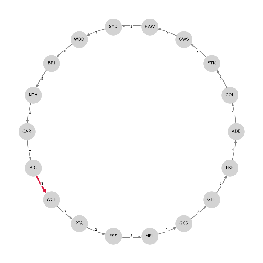
Nothing separates the two solves but the labels: 2 May 2026 is a round 8 fixture, so both name the same moment, one to the round and one to the day. Reading the chain off, with the round in which each link was established:
>>> for position, team in enumerate(result.cycle):
...     beaten = result.cycle[(position + 1) % len(result.cycle)]
...     print(f"{team} beat {beaten} in round {result.weights[position]}")
ADE beat COL in round 1
COL beat STK in round 0
STK beat GWS in round 2
GWS beat HAW in round 0
HAW beat SYD in round 2
SYD beat WBD in round 7
WBD beat BRI in round 0
BRI beat NTH in round 5
NTH beat CAR in round 4
CAR beat RIC in round 1
RIC beat WCE in round 8
WCE beat PTA in round 3
PTA beat ESS in round 2
ESS beat MEL in round 5
MEL beat GCS in round 4
GCS beat GEE in round 0
GEE beat FRE in round 1
FRE beat ADE in round 4
Every other link was in place well before round 8. The single arc holding the
whole circle back is RIC beat WCE, Richmond’s first win of the season, and
the game played on the very day the calendar solve returned.
Looking forward from mid-season
The same model answers the live version of the question. Suppose we are five rounds in, and want to know the earliest the circle could still be completed and which results would have to go our way. Only the input changes, and since this page has a completed season to hand, the results that had not happened yet have to be taken back out of it:
def as_at(season, played_through):
    """The season as it stood at the end of ``played_through``: the later
    games are still on the fixture, but their results are not known yet."""
    return season.assign(
        winner=season["winner"].mask(season["round"] > played_through)
    )
>>> partial = min_bottleneck_hamiltonian_cycle(
...     build_arcs(as_at(season, 5)), verbose=False
... )
>>> partial.bottleneck
6
After five rounds it still looked possible to close the circle in round 6. That would have needed seven specific results, which the solution names:
>>> for position, team in enumerate(partial.cycle):
...     if partial.weights[position] > 5:
...         beaten = partial.cycle[(position + 1) % len(partial.cycle)]
...         print(f"{team} must beat {beaten} in round {partial.weights[position]}")
COL must beat CAR in round 6
RIC must beat NTH in round 6
ESS must beat GCS in round 6
GEE must beat WBD in round 6
WCE must beat FRE in round 6
MEL must beat BRI in round 6
STK must beat ADE in round 6
They did not all go that way, and the answer drifted later as the season wore on. This is not a coincidence: learning a result only ever removes arcs, as two possible orientations collapse into the one that actually happened, or into none at all if the game was drawn. The set of available cycles can only shrink, so the earliest possible completion can only move later:
>>> for played_through in range(-1, 8):
...     answer = min_bottleneck_hamiltonian_cycle(
...         build_arcs(as_at(season, played_through)), verbose=False
...     ).bottleneck
...     print(f"after round {played_through:2d}:  earliest completion is round {answer}")
after round -1:  earliest completion is round 3
after round  0:  earliest completion is round 3
after round  1:  earliest completion is round 4
after round  2:  earliest completion is round 4
after round  3:  earliest completion is round 5
after round  4:  earliest completion is round 5
after round  5:  earliest completion is round 6
after round  6:  earliest completion is round 7
after round  7:  earliest completion is round 8
The first line is the pre-season case, where nothing has been played and every game in the fixture offers both orientations. Purely as a matter of scheduling, the 2026 fixture could not have produced a circle of parity before round 3, no matter how the results fell. By round 7 the answer had settled on round 8, which is where it stayed.
The circle can be drawn with the teams laid out in cycle order:
import matplotlib.pyplot as plt
import networkx as nx

graph = nx.DiGraph()
for position, team in enumerate(result.cycle):
    beaten = result.cycle[(position + 1) % len(result.cycle)]
    graph.add_edge(team, beaten, when=result.weights[position])

layout = nx.circular_layout(graph)
latest = [
    (u, v) for u, v, w in graph.edges(data="when") if w == result.bottleneck
]

fig, ax = plt.subplots(figsize=(8, 8))
nx.draw_networkx_nodes(graph, layout, ax=ax, node_size=1300, node_color="lightgray")
nx.draw_networkx_labels(graph, layout, ax=ax, font_size=9)
nx.draw_networkx_edges(graph, layout, ax=ax, node_size=1300, width=1.5,
               edge_color="gray", connectionstyle="arc3,rad=0.08")
nx.draw_networkx_edges(graph, layout, ax=ax, node_size=1300, width=3.0,
               edgelist=latest, edge_color="crimson",
               connectionstyle="arc3,rad=0.08")
nx.draw_networkx_edge_labels(
    graph, layout, ax=ax, font_size=8, rotate=False,
    bbox={"boxstyle": "round,pad=0.15", "fc": "white", "ec": "none"},
    edge_labels=nx.get_edge_attributes(graph, "when"),
)
ax.set_axis_off()
fig.tight_layout()
plt.show()
Each arrow points from the winner to the loser and is labeled with the weight of that link, here the round in which the result occurred. The red arrow is the bottleneck: the last link to fall into place, and the one that determines when the circle closed.