Metro Map: Computing an Octilinear Graph Representation
A metro map is a schematic drawing of metro lines with stations and transfer stations. A schematic graph drawing aims to ease navigation, such as how to get from A to B in a transportation network. There are several different requirements for a schematic graph drawing. In this OptiMod, we will consider an octilinear representation, i.e., the edges of the network are restricted to horizontals, verticals, and diagonals at 45 degrees. Such a schematic drawing is of special interest when showing metro lines, but could also be useful for general transportation networks or graphs. Note that an octilinear representation requires a maximum vertex degree of eight. If satisfied, this OptiMod computes an octilinear representation for any undirected graph. The original geographical information of the graph is included. More precisely, the geographical information defines an input embedding, which is preserved in the schematic representation. The mathematical formulation is based on the one given by Nöllenburg [1]. This diploma thesis provides additional detailed descriptions and explanations. However, we slightly changed some variable types and, hence, some constraints.
Problem Specification
Let \(G\) be an undirected graph with a set of nodes \(V\) and edges \(E\). For each node, a geographical position is given as x- and y-coordinates.
In the octilinear representation, the edge can be drawn in eight different directions when fixing one of its endpoints. Considering the edge \((u,v)\in E\), the node \(v\) can be in the east, north-east, north, north-west, west, south-west, south, or south-east of \(u\). We enumerate these directions from 0 to 7, starting with the east and traversing the directions counter-clockwise. The figure below shows the idea. Assume the node \(u\) is positioned in the center. The edge \((u,v)\) can follow the directions 0 to 7 that represent the cardinal directions.
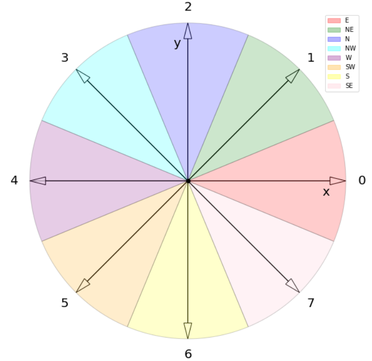
Idea of the octilinear representation. Assuming a node \(u\) in the center, an edge \((u,v)\) can be drawn in directions 0 to 7.
Based on the directions, we can determine conditions on the coordinates. For example, if the direction of \((u,v)\) is 0, then \(u\) and \(v\) have the same y-coordinate while the x-coordinate of \(v\) must be at least one larger than the one of \(u\).
In this OptiMod, an octilinear graph representation is computed. More precisely, for each edge, a direction (0 to 7) is computed, and all nodes are assigned to x- and y-coordinates that support the edge directions. Additionally, the following is considered
The original positions of the nodes are respected in the following way:
Only directions that align with the original direction or are directly neighbored are allowed. For example, if \(v\) is north-east (1) from \(u\) in the original positions, it is allowed to place v north, north-east, or east in the octilinear representation, i.e., for the edge \((u,v)\) the directions 2, 1, and 0 are allowed.
The ordering of all adjacent nodes of a node \(v\) is preserved.
The distance (difference in x- or y-coordinate) between each two nodes is at least one and as minimal as possible
If a set of paths in the graph is given (representing, for example, metro lines), the bends along the lines are minimized.
If possible, ensure planarity.
Some remarks about planarity: The number of constraints to ensure planarity is quadratic in the number of edges of the graph. Hence, the planarity part is the largest part of the model. Instead of adding all the constraints initially, we use a callback approach and lazily add these constraints, i.e., only when they are violated. Moreover, the planarity restrictions are included as soft constraints, i.e., if there is no planar representation, an embedding with the fewest planarity violations is computed. There is an option to turn off the planarity requirement. The restrictions from the origin geographical positions often imply a planar solution without including planarity constraints. In these cases, the performance can be improved if planarity constraints are not considered.
We consider three weights to balance the different parts of the objective. The weight \(w_o\) is a penalty for a direction of an edge \((u,v)\). More precisely, it penalizes the direction if \(v\) is not placed in the original but at a neighboring direction. The weight \(w_d\) penalizes a distance of an edge greater than a minimum distance of one, and \(w_b\) penalizes the line bends. These three weights have a default value of 1 but are parameterized and can be adapted. Additionally, the planarity violations are included in the objective. They are weighted with 1000. This should be considered when choosing weights for \(w_o\), \(w_d\), and \(w_b\); we restrict the values to be between 0 and 100.
Background: Mathematical Formulation
This OptiMod is implemented by formulating a mixed integer program and solving it using Gurobi. Instead of presenting the complete formulation as a whole (which is too bulky), the different aspects of the model are discussed below.
Variables
We use the following variables:
\(d(u,v,r)\in\{0,1\}\) for \((u,v)\in E\) and \(r\in\{0,1,\ldots,7\}\) which indicates whether the direction from \(u\) to \(v\) is \(r\).
\(x(v) \geq 0\) the x-coordinate of node \(v\) in an octilinear representation
\(y(v) \geq 0\) the y-coordinate of node \(v\) in an octilinear representation
\(\delta(u,v)\geq 0\) the distance of \(u\) and \(v\) for each edge \((u,v)\in E\) that is larger than the minimum required distance of 1
\(b(u,v,w,i)\in\{0,1\}\) the bend of category \(i\) on two adjacent edges \((u,v), (v,w)\in E\). The category corresponds to the angle of the bend. The angle can be equal to 180 (=category 0), 135 (=category 1), 90 (=category 2), and 45 degrees (=category 3).
Objective Function
The objective minimizes a weighted sum of
the distances,
the directions that do not correspond to the original directions (here indicated by the set \(J_{uv}\) for an edge \((u,v)\in E\)),
and the bends for each line weighted by its bend category, i.e., the cost increases with the acuteness of the angle. Here \(|L_{u,v,w}|\) amounts the number of lines traversing the adjacent edges \((u,v),(v,w)\in E\).
These three parts are weighted by \(w_d\), \(w_o\), and \(w_b\). Note that the direction variables \(d(u,v,j)\) for all directions \(j\) not equivalent to the original direction, or their direct neighbors are set to 0.
The penalization of planarity violations is omitted here for ease of notation but briefly discussed in the planarity section.
Direction Variables and Coordinates
We ensure that the direction from \(u\) to \(v\) matches the reverse direction from \(v\) to \(u\).
The next constraint requires that exactly one directions is chosen for each edge.
Finally, we have constraints to define the conditions on the x- and y-coordinates that need to be satisfied if a certain direction is chosen for the edge.
Note that the minimum distance between two different nodes need to be 1 in either x- or y-coordinate. To ensure this for diagonal directions we need to require a right-hand-side of 2.
Edge Order
To ensure the preservation of the original edge order, it is sufficient to consider all nodes that have at least two adjacent nodes. We need auxiliary binary variables \(\beta_v^i\) for each such node \(v\) and each adjacent node \(i\) of \(v\). Let the adjacent nodes of \(v\) be ordered counter-clockwise and assume that \(w_0,\ldots, w_{\deg(v)}\) fulfills this order. Then also in the octilinear representation the nodes need to have the same counter-clockwise order, i.e., the direction from neighbor node \(i\) to \(i+1\) increases with at most one exception (when switching from direction 7 to 0). For this exception we allow \(\beta_v^i\) to be 1. The following constraints define the requirement.
Distance
The minimum distance between two nodes of one edge is 1 in either x- or y-coordinate. This is ensured via constraints, see section on Direction Variables and Coordinates. The distance variables count every additional distance in x- and y-coordinates.
Line Bends
Whenever, a line traverses the adjacent edges \((u,v)\) and \((v,w)\), we want to amount the bend of the two edges in the octilinear representation. There are four possibilities reflected by the variables \(b(u,v,w,0)\) (no bend, 180 degrees), \(b(u,v,w,1)\) (a bend of 135 degrees), \(b(u,v,w,2)\) (a bend of 90 degrees), and \(b(u,v,w,3)\) (a bend of 45 degrees). The following constraints ensure that exactly one of these variables is chosen and that the bend in direction \(u,v,w\) is equal to the bend in direction \(w,v,u\).
The angle or the bend category can be determined from the direction variables of the edges. The following constraints require that the directions of the edges \((u,v)\) and \((v,u)\) match the bend variable.
Planarity
To guarantee planarity we have to ensure that pairs of edges do not intersect. Again, we use the eight possible directions to express which direction an edge \(e2\) is relative to an edge \(e1\). For example, fixing the position of edge \(e1\) the second edge \(e2\) must be placed east, east-north, north, north-west, west, south-west, south, or south-east of \(e1\).
We define variables that express this positional relation between each two edges. Let \(\gamma(u1,v1,u2,v2,i) \in\{0,1\}\) be a binary variable that indicate that edge \((u2,v2)\in E\) is positioned in direction \(i\) from edge \((u1,v1)\). We add an additional variable \(\gamma(u1,v1,u2,v2)^o \in\{0,1\}\) to capture non-planarity for these two edges. This variable is added with a cost of 1000 to the objective function.
In this way, either a planarity violation is counted or one of the other planarity variables need to be chosen which implies conditions on the positions of the nodes of the edges. As an example, we only present the constraints for the condition that edge \((u2,v2)\in E\) is positioned in direction 3 (north-west) from edge \((u1,v1)\).
The constraints need to be defined for all directions and for each two non-adjacent edges. We include these constraints as lazy constraints in a callback function. Note that indicator constraints cannot be added in a callback function. Hence, we define these constraints as big-M constraints.
Improving Constraints
The IP model is well-defined with the above-discussed constraints. However, we want to add some further constraints to slightly improve the LP relaxation and the performance of the optimization.
The first constraint ensures that each direction is chosen only once for all edges adjacent to \(v\)
Inspired by the fact that geographical restrictions allow only three possible directions for each edge, we can observe the following. If, for example, only the directions 0, 1, and 2 are allowed for an edge \((u,v)\), i.e., \(d(u,v,3)=d(u,v,4)=d(u,v,5)=d(u,v,6)=d(u,v,7)=0\), we are in the positive part of the coordinate system and the following constraints must hold
Similar constraints result when considering all other combinations of 3 adjacent directions. We add these conditions as big-M constraints to the model and use an epsilon of 1e-6 (=feasibility tolerance) to handle the strict inequality.
For the bend variables, the following constraint can be added
The constraint states that edge \((u,v)\) can have a bend of 0 with at most one of its adjacent edges.
All these improving constraints are added by default. However, a parameter
improve_lp is provided that can be set to False and then these improving
constraints are not added.
Code and Inputs
For this OptiMod, the networkx package is needed. The input is a
networkx graph for the network information and a pd.DataFrame for the line
information. The output is a networkx graph with node property pos_oct
representing the x-and y-coordinates for the octilinear representation and a
Python dictionary for the direction of each edge.
An example of the inputs with the respective requirements is shown below.
>>> import networkx as nx
>>> from gurobi_optimods import datasets
>>> graph, linepath_data = datasets.load_berlin_metro_reduced_graph_data()
>>> print(graph)
  Graph with 29 nodes and 32 edges
>>> pos_orig = nx.get_node_attributes(graph, 'pos')
>>> len(pos_orig)
  29
>>> linepath_data.head(4)
  linename  edge_source     edge_target
  0       U1         147          50
  1       U1          50          82
  2       U1          82         127
  3       U1         127          53
For the example, we used data from the Berlin metro network. For demonstration,
we use only a small part of the whole network. The graph includes
the node attribute pos that contains a tuple of x- and y-coordinates for
the original position. The linepath_data must be consistent with
the graph. For example, edge_source, edge_target in the
linepath_data must correspond to the node names in the graph.
Solution
The output of the optimization is the following:
A graph with the node attribute
pos_octcontaining the x- and y-coordinates for the octilinear representation. It also contains the original node attributeposwith the original positions.A Python dictionary providing the direction (0 to 7) for each edge. This information is needed for the plotting function provided in the OptiMod
The OptiMod can be run as follows:
>>> from gurobi_optimods import datasets
>>> from gurobi_optimods.metromap import metromap
>>> graph, linepath_data = datasets.load_berlin_metro_reduced_graph_data()
>>> graph_out, edge_directions = metromap(
...     graph,
...     linepath_data,
...     include_planarity=False,
...     improve_lp=False,
...     verbose=False
... )
>>> # Show that input and output graphs are isomorphic (structural equivalent)
>>> import networkx as nx
>>> print(nx.is_isomorphic(graph, graph_out))
  True
>>> # Show the first 4 nodes with their attributes
>>> first_four_nodes_with_attrs = list(graph_out.nodes.data())[:4]
>>> print(first_four_nodes_with_attrs)
[(50, {'pos': [13.428468, 52.499035], 'pos_oct': (5.0, 3.0)}),
 (82, {'pos': [13.417748, 52.499047], 'pos_oct': (4.0, 3.0)}),
 (127, {'pos': [13.406531, 52.498274], 'pos_oct': (3.0, 3.0)}),
 (53, {'pos': [13.39176, 52.497774], 'pos_oct': (1.0, 3.0)})]
Note, for this demonstration the parameter include_planarity is set to
False, and we skip the improving constraints. This is done so that the test
works with the Gurobi test license. For this example, the planarity constraints
are usually satisfied. If the planarity constraints should be included in the
computation, the parameter include_planarity can be omitted or set to True.
If a full Gurobi license is available, the full Berlin metro network can be
loaded and tested with datasets.load_berlin_metro_graph_data().
The graph can be plotted using the networkx plotting function, for example, as follows:
pos_oct=nx.get_node_attributes(graph_out, "pos_oct")
nx.draw(
    graph_out,
    pos_oct,
    with_labels=False,
    node_size=12,
    edgecolors="black",
    node_color="white",
)
As a comparison the original node positions can be plotted as well:
pos_orig=nx.get_node_attributes(graph, "pos")
nx.draw(
    graph,
    pos_orig,
    with_labels=False,
    node_size=12,
    edgecolors="black",
    node_color="white",
)
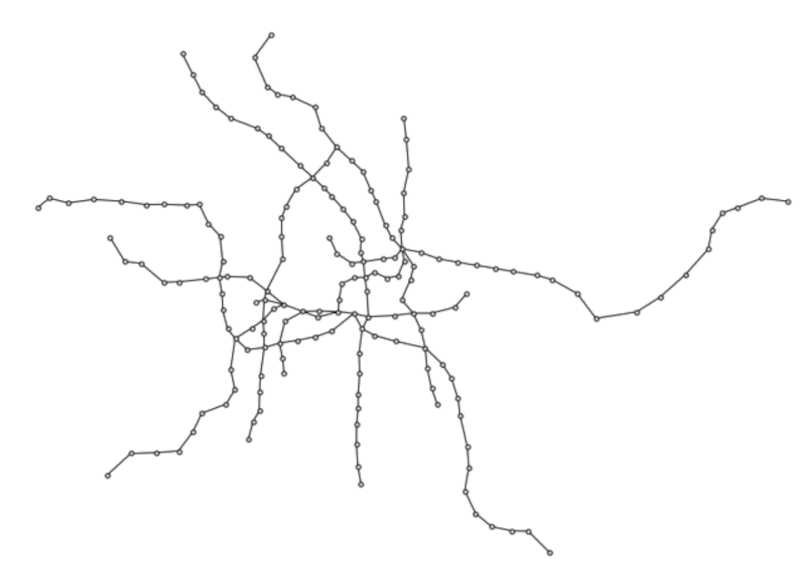
Below is a networkx plot of the graph with the original positions (left) and
the computed octilinear positions (right) for the Berlin metro network. First
the small part is shown and below the full network.
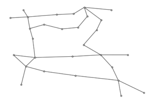
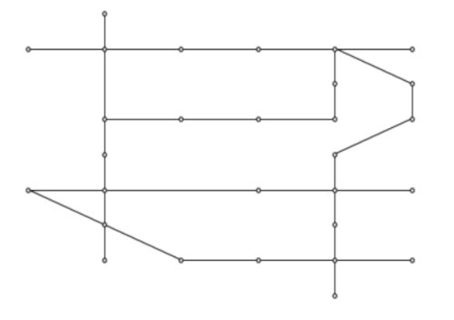
Note that optimizing the small subnetwork does not include restrictions coming from other parts of the network. Therefore, an optimal solution is often different for this subnetwork than when considered in the complete network.
We provide a method to plot the lines in the octilinear representation using plotly.
In order to use this functionality, the plotly package is needed.
The plot function generates a plot that is opened in a browser. The lines can be turned off and on in this plot when clicking the respective name in the legend. The plot function can be called as follows:
from gurobi_optimods.metromap import plot_map
plot_map(graph_out, edge_directions, linepath_data)
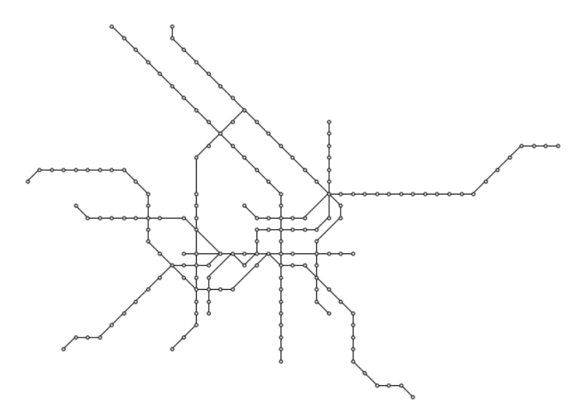
The following figure is an example of the above call, it shows the lines in the octilinear representation of the Berlin metro network. (Use link to open in full screen.)
Note that plotting the lines in the octilinear network is an art or a further optimization problem. If lines share an edge, it needs to be decided how to shift the lines so that both can be distinguished, which is above, below, left, or right, and which colors should be used. The plotting function that is provided in this OptiMod is not very sophisticated. Feel free to contribute with improvement ideas.
Parameter: Planarity and Objective Function
As already mentioned, it is possible to change the weights in the objective or
omit the planarity restrictions. The planarity parameter was already considered
in the solve example. The default value is true, i.e., if the parameter is not
set when calling the metromap function, the planarity constraints are
included via a callback function.
Similar holds for the weights of the different parts in the objective. The default value for all weights is 1. If a different weighting is requested, this can be done as follows:
graph_out, edge_directions = metromap(
    graph,
    linepath_data,
    penalty_edge_directions=2,
    penalty_line_bends=0,
    penalty_distance=1,
)
Combination with Line Optimization OptiMod
After computing an optimal line plan with the Line Optimization OptiMode, an octilinear representation and the corresponding metromap can be computed with this OptiMod. Here is an example of how this could be done
# import all requirements
import networkx as nx
from gurobi_optimods import datasets
from gurobi_optimods.line_optimization import line_optimization
from gurobi_optimods.metromap import metromap
from gurobi_optimods.metromap import plot_map

# load data for line optimization and compute line plan
node_data, edge_data, line_data, linepath_data, demand_data = (
    datasets.load_siouxfalls_network_data()
)
frequencies = [1, 3]
obj_cost, final_lines = line_optimization(
    node_data,
    edge_data,
    line_data,
    linepath_data,
    demand_data,
    frequencies,
    verbose=False,
)
# create a data frame containing only the linepaths of the solution
linepath_data_sol = linepath_data[
    linepath_data["linename"].isin([line for line, freq in final_lines])
]
# create networkx graph
graph = nx.from_pandas_edgelist(
    edge_data.reset_index(), create_using=nx.Graph()
)
# add x-, y-coordinates as node attribute
for number, row in node_data.set_index("number").iterrows():
    graph.add_node(number, pos=(row["posx"], row["posy"]))
# compute and plot metromap
graph_out, edge_directions = metromap(
  graph, linepath_data_sol, penalty_line_bends=0, verbose=False)
plot_map(graph_out, edge_directions, linepath_data_sol)
Further Remarks
It is possible to compute an octilinear representation of a graph without
providing a set of lines. Of course, line bends are then not considered in the
objective. The linepath_data parameter can be omitted in this case:
graph_out, edge_directions = map.metromap(graph)
It is also possible to provide a graph without any information about the
original positions, i.e., without the node attribute pos. In this case, all
directions for an edge are allowed, and no direction is penalized. Moreover,
there is no given edge order that needs to be preserved. However, note that in
this case, the problem usually becomes much harder to solve. A different approach
or a strengthened model formulation might be necessary to solve medium-sized
problems to optimality if no further restrictions from original positions are
given.