Least Absolute Deviation Regression

Least Absolute Deviation (LAD) regression is an alternative to the more commonly used Ordinary Least Squares (OLS) regression method. The distinction between the two is the error metric used to fit the predictive model to training data. LAD minimizes the sum of absolute residuals, while OLS minimizes the sum of squares of residuals.

Though most machine learning practitioners are probably more familiar with OLS, LAD was proposed around 50 years earlier [1]. OLS gained more popularity partly due to the fact that the computations required were simpler. It was the development of linear programming that made LAD computationally manageable [2].

LAD is more robust than OLS in that it is more resistant to outliers in the response variable [1]. In OLS, a large residual for a single data point makes an outsized contribution to the loss function since the residuals are squared. As a result, a single outlier can have a large effect on the fitted coefficients and skew the resulting model. By contrast, a large deviation in an individual point has a less extreme effect on the linear loss function of LAD.

Problem Specification

Scikit-learn’s documentation gives a general explanation of Linear Models. The distinction between this Mod and the Ordinary Least Squares regression algorithm from scikit-learn is the loss function. LADRegression chooses coefficients \(w\) of a linear model \(y = Xw\) so as to minimize the sum of absolute errors on a training dataset \((X, y)\). In other words, it aims to minimize the following loss function:

\[\min_w \lvert Xw - y \rvert\]

Background: Mathematical Model

The fitting algorithm of the LAD regression Mod is implemented by formulating the loss function as a Linear Program (LP), which is then solved using Gurobi. Here \(I\) is the set of observations and \(J\) the set of fields. Response values \(y_i\) are predicted from predictor values \(x_{ij}\) by fitting coefficients \(w_j\). To handle the absolute value in the loss function, auxiliary non-negative variables \(u_i\) and \(v_i\) are introduced.

\[\begin{split}\begin{alignat}{2} \min \quad & \sum_i u_i + v_i \\ \mbox{s.t.} \quad & \sum_j w_j x_{ij} + u_i - v_i = y_i \quad & \forall i \in I \\ & u_i, v_i \ge 0 \quad & \forall i \in I \\ & w_j \,\, \text{free} \quad & \forall j \in J \\ \end{alignat}\end{split}\]

Example Code

This Mod implements the fit-predict API used by all predictive models in scikit-learn (including the sklearn.linear_model.LinearRegression class). The example below reads in the diabetes dataset from scikit-learn, performs a train-test split, fits a LAD regression model to the training data, and creates predictions for the testing data.

from sklearn import datasets
from sklearn.model_selection import train_test_split

from gurobi_optimods.regression import LADRegression

# Load the diabetes dataset
diabetes = datasets.load_diabetes()

# Split data for fit assessment
X_train, X_test, y_train, y_test = train_test_split(
    diabetes["data"], diabetes["target"], random_state=42
)

# Fit model and obtain predictions
lad = LADRegression()
lad.fit(X_train, y_train)
y_pred = lad.predict(X_test)

Note that the input data is provided as numpy arrays. For a dataset containing n observations and m independent variables, feature datasets X_train and X_test have shape (n, m), while response variable datasets y_train and y_test have shape (n,).

>>> X_train.shape
(331, 10)
>>> y_train.shape
(331,)
>>> X_test.shape
(111, 10)
>>> y_test.shape
(111,)

Comparison with Ordinary Least Squares

Here we extract the coefficients of the fitted model and compare them with the coefficients found using Ordinary Least Squares (OLS).

import pandas as pd
import matplotlib.pyplot as plt
from sklearn.linear_model import LinearRegression

ols = LinearRegression()
ols.fit(X_train, y_train)
coefficients = pd.DataFrame(
    data={"OLS": ols.coef_, "LAD": lad.coef_},
    index=diabetes["feature_names"],
)

plt.figure(figsize=(8, 4))
coefficients.plot.bar(ax=plt.gca())

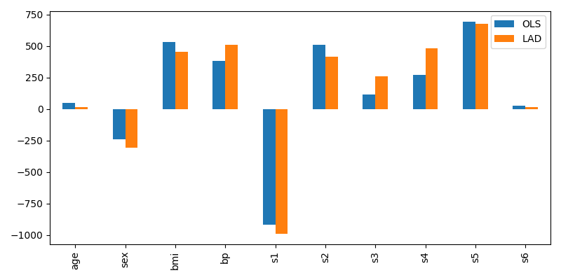
At this stage there isn’t much to observe; the chosen coefficients are similar:

Comparison of regression coefficients fitted by LAD and OLS

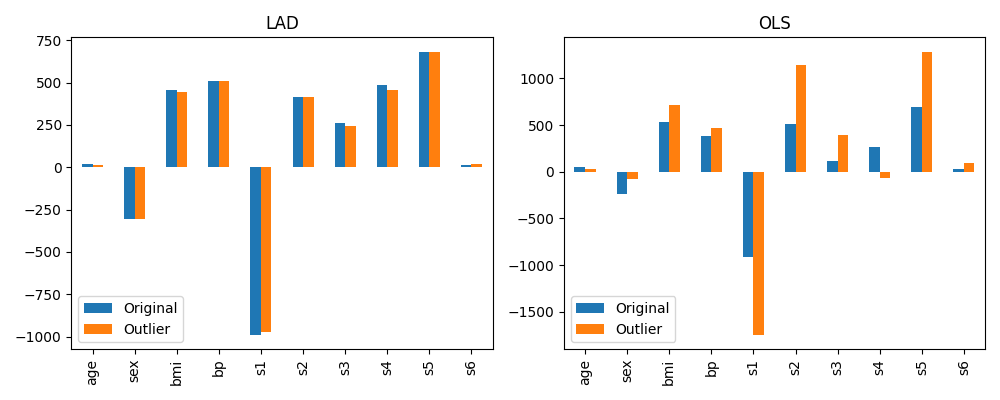
Things get more interesting when we analyze the impact of outliers in the training dataset on the resulting coefficients and performance of the model. In this contrived test, outliers are introduced into the training data by scaling a small number of entries in y_train (4 of 331 response variables values are scaled by a factor of 5). Both LAD and OLS models are fitted to this altered training set, and the resulting models are compared to the original fitted models.

View the code: resistance to outliers comparison figures

from sklearn.metrics import mean_absolute_error, mean_squared_error

# Introduce some (admittedly absurd) scaling to produce
# outliers in one training set
y_train_outliers = y_train.copy()
y_train_outliers[[14, 78, 234, 123]] *= 5

# Fit both model types to both training sets, and evaluate
# test set errors
models = [
    {"regressor": cls(), "y_train": y, "name": name, "label": label}
    for cls, name in [(LADRegression, "LAD"), (LinearRegression, "OLS")]
    for y, label in [(y_train, "Original"), (y_train_outliers, "Outlier")]
]
for model in models:
    model["regressor"].fit(X_train, model["y_train"])
    y_pred = model["regressor"].predict(X_test)
    model["mae-test"] = mean_absolute_error(y_test, y_pred)
    model["mse-test"] = mean_squared_error(y_test, y_pred)

# Plot coefficients trained on the original and outlier sets
coeffs = pd.DataFrame(
    data={
        (model["name"], model["label"]): model["regressor"].coef_
        for model in models
    },
    index=diabetes['feature_names'],
)
fig, (ax1, ax2) = plt.subplots(1, 2, figsize=(10, 4))
coeffs["LAD"].plot.bar(ax=ax1, title="LAD")
ax1.legend(loc='lower left')
coeffs["OLS"].plot.bar(ax=ax2, title="OLS")
ax2.legend(loc='lower left')

# Plot test set errors
errors = pd.DataFrame(models)
fig, (ax1, ax2) = plt.subplots(1, 2, figsize=(10, 4))
errors.set_index(["name", "label"])["mae-test"].unstack().plot.bar(
    ax=ax1, xlabel="", title="Mean Absolute Error (test set)"
)
ax1.legend(loc='lower left')
errors.set_index(["name", "label"])["mse-test"].unstack().plot.bar(
    ax=ax2, xlabel="", title="Mean Squared Error (test set)"
)
ax2.legend(loc='lower left')

The figure below compares the model coefficients trained on the original set and the outlier training set for each model type. We can see that the OLS model is much more significantly affected by the introduction of outliers. The dominant coefficients have approximately doubled in some cases, and some smaller coefficients have even reversed their sign. By comparison, the LAD model is almost unchanged by the introduction of these few outliers.

Effect of training set outliers on LAD and OLS model coefficients

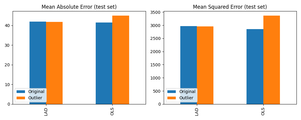
Finally, we compare the mean absolute error (MAE) and mean squared error (MSE) metrics of each fitted model on the test set. This measures the ability of each model to generalise to data points not part of the training set. Of note here is that the OLS model shows significantly higher errors on the test set when trained on the outlier dataset. By comparison, LAD model performance is almost unchanged. Thus, as expected, the LAD model is much more robust to training set outliers than the OLS model.

Effect of training set outliers on LAD and OLS test set errors

[1] (1,2)

David Birkes and Yadolah Dodge. Alternative methods of regression. John Wiley & Sons, 2011.

[2]

Peter Bloomfield and William Steiger. Least absolute deviations curve-fitting. SIAM Journal on scientific and statistical computing, 1(2):290–301, 1980.