Maximum Flow / Minimum Cut
The maximum flow problem finds the total flow that can be routed through a capacitated network from a given source vertex to a given sink vertex. The minimum cut problem finds a set of edges in the same graph with minimal combined capacity that, when removed, would disconnect the source from the sink. The two problems are related through duality: the maximum flow is equal to the capacity of the minimum cut.
The first algorithm proposed to solve this problem was the Ford-Fulkerson algorithm [1]. Goldberg and Tarjan[2] later proposed the famous push-relabel algorithm, and more recently, Orlin[3] and other authors have proposed polynomial-time algorithms. The maximum flow problem is a special case of the minimum cost flow problem, so it can also be solved efficiently using the network simplex algorithm [4] making a linear programming (LP) solver a suitable approach.
Problem Specification
Let \(G\) be a graph with set of vertices \(V\) and edges \(E\). Each edge \((i,j)\in E\) has capacity \(B_{ij}\in\mathbb{R}\). Given a source vertex \(s\in V\) and a sink vertex \(t\in V\) the two problems can be stated as follows:
Maximum Flow: Find the flow with maximum value from source to sink such that the flow is capacity feasible.
Minimum Cut: Find the set of edges which disconnects the source and sink such that the total capacity of the cut is minimised.
Background: Optimization Model
Let us define a set of continuous variables \(x_{ij}\) to represent the amount of non-negative (\(\geq 0\)) flow going through an edge \((i,j) \in E\).
The mathematical formulation for the maximum flow can be stated as:
where \(\delta^+(\cdot)\) (\(\delta^-(\cdot)\)) denotes the outgoing (incoming) neighbours of a given vertex.
The objective maximises the total outgoing flow from the source vertex. The first set of constraint ensure flow balance for all vertices. That is, for a given node that is neither the source or the sink, the outgoing flow must be equal to the incoming flow. The last set of constraints ensure non-negativity of the variables and that the capacity of each edge is not exceeded.
The minimum cut problem formulation is the dual of the maximum flow formulation. The minimum cut is found by solving the maximum flow problem and extracting the constraint dual values. Specifically, the edges in the cutset are those whose capacity constraints have non-zero dual values. The graph partitions formed by removing the edges in the cutset can then be round by following the predecessor and successor vertices of these edges.
Code and Inputs
This Mod accepts input graphs of any of the following types:
pandas: using a
pd.DataFrame;NetworkX: using a
nx.DiGraphornx.Graph;SciPy.sparse: using a
sp.sparraymatrix.
An example of these inputs with their respective requirements is shown below.
>>> from gurobi_optimods import datasets
>>> edge_data, _ = datasets.simple_graph_pandas()
>>> edge_data[["capacity"]]
               capacity
source target
0      1              2
       2              2
1      3              1
2      3              1
       4              2
3      5              2
4      5              2
The edge_data DataFrame is indexed by source and target nodes
and contains columns labelled capacity with the edge attributes.
>>> from gurobi_optimods import datasets
>>> G = datasets.simple_graph_networkx()
>>> for u, v, capacity in G.edges.data("capacity"):
...     print(f"{u} -> {v}: {capacity = }")
0 -> 1: capacity = 2
0 -> 2: capacity = 2
1 -> 3: capacity = 1
2 -> 3: capacity = 1
2 -> 4: capacity = 2
3 -> 5: capacity = 2
4 -> 5: capacity = 2
Edges have attributes capacity.
>>> from gurobi_optimods import datasets
>>> G, capacities, _, _ = datasets.simple_graph_scipy()
>>> G.data = capacities.data # Copy capacity data
>>> for edge, value in zip(zip(*G.coords), G.data):
...     print(f"{edge}:  {value}")
  (0, 1):  2
  (0, 2):  2
  (1, 3):  1
  (2, 3):  1
  (2, 4):  2
  (3, 5):  2
  (4, 5):  2
We only need the adjacency matrix for the graph (as a sparse array) where each each entry contains the capacity of the edge.
Solution
Maximum Flow
Let us use the data to solve the maximum flow problem.
>>> from gurobi_optimods.max_flow import max_flow
>>> obj, flow = max_flow(edge_data, 0, 5, verbose=False) # Find max-flow between nodes 0 and 5
>>> obj
3.0
>>> flow
source  target
0       1         1.0
        2         2.0
1       3         1.0
2       3         1.0
        4         1.0
3       5         2.0
4       5         1.0
Name: flow, dtype: float64
The max_flow function returns the value of the maximum flow as well as
a pd.Series with the flow per edge. Similarly as the input DataFrame
the resulting series is indexed by source and target. In this
case, the resulting maximum flow has value 3.
>>> from gurobi_optimods.max_flow import max_flow
>>> obj, sol = max_flow(G, 0, 5, verbose=False)
>>> obj
3.0
>>> type(sol)
<class 'networkx.classes.digraph.DiGraph'>
>>> list(sol.edges(data=True))
[(0, 1, {'flow': 1.0}), (0, 2, {'flow': 2.0}), (1, 3, {'flow': 1.0}), (2, 3, {'flow': 1.0}), (2, 4, {'flow': 1.0}), (3, 5, {'flow': 2.0}), (4, 5, {'flow': 1.0})]
The max_flow function returns the value of the maximum flow as well as
a dictionary indexed by edge with the non-zero flow.
>>> from gurobi_optimods.max_flow import max_flow
>>> obj, sol = max_flow(G, 0, 5, verbose=False)
>>> obj
3.0
>>> for edge, value in zip(zip(*sol.coords), sol.data):
...     print(f"{edge}:  {value}")
  (0, 1):  1.0
  (0, 2):  2.0
  (1, 3):  1.0
  (2, 4):  2.0
  (3, 5):  1.0
  (4, 5):  2.0
The max_flow function returns the value of the maximum flow as well a
sparse array with the amount of non-zero flow in each edge in the
solution.
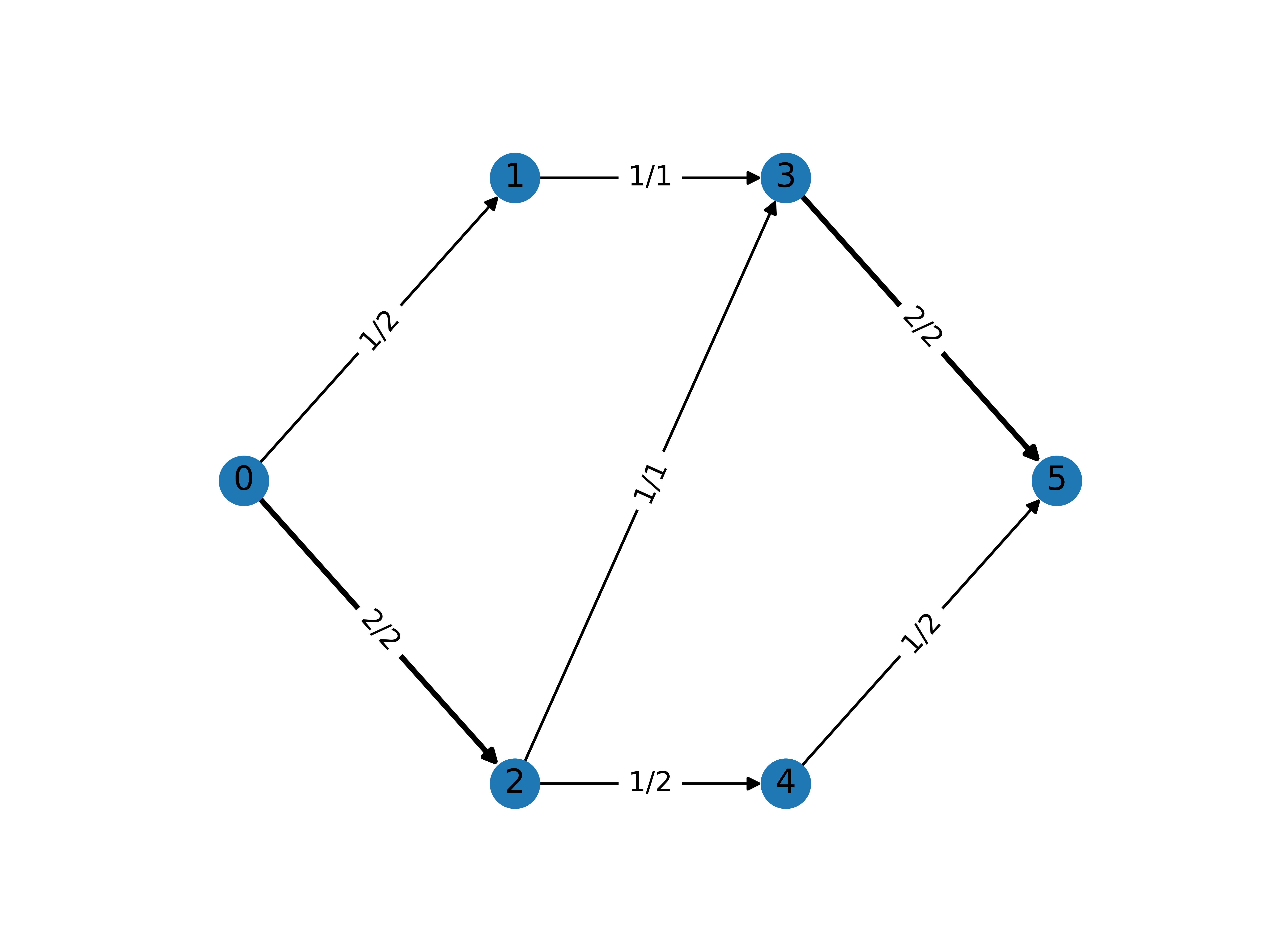
The solution for this example is shown in the figure below. The edge labels denote the edge capacity and resulting flow: \(x^*_{ij}/B_{ij}\). All edges in the maximum flow solution carry some flow, totalling at 3.0 at the sink.

Minimum Cut
Let us use the data to solve the minimum cut problem.
>>> from gurobi_optimods.min_cut import min_cut
>>> res = min_cut(edge_data, 0, 5, verbose=False)
>>> res
MinCutResult(cut_value=3.0, partition=({0, 1}, {2, 3, 4, 5}), cutset={(0, 2), (1, 3)})
>>> res.cut_value
3.0
>>> res.partition
({0, 1}, {2, 3, 4, 5})
>>> res.cutset
{(0, 2), (1, 3)}
The min_cut function returns a MinCutResult which contains the
cutset value, the partition of the nodes and the edges in the cutset.
>>> from gurobi_optimods.min_cut import min_cut
>>> res = min_cut(G, 0, 5, verbose=False)
>>> res
MinCutResult(cut_value=3.0, partition=({0, 1}, {2, 3, 4, 5}), cutset={(0, 2), (1, 3)})
>>> res.cut_value
3.0
>>> res.partition
({0, 1}, {2, 3, 4, 5})
>>> res.cutset
{(0, 2), (1, 3)}
The min_cut function returns a MinCutResult which contains the
cutset value, the partition of the nodes and the edges in the cutset.
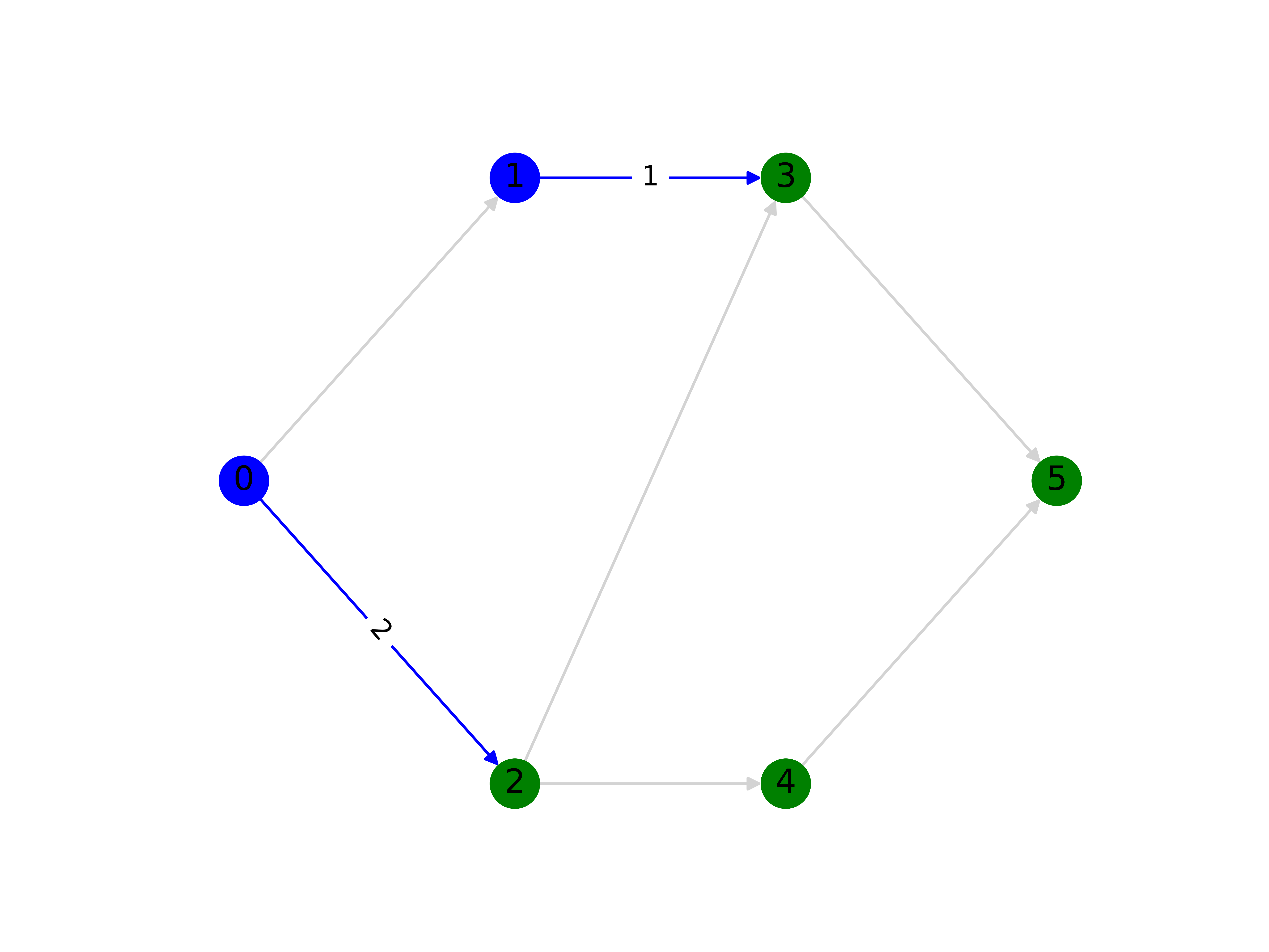
The solution for the minimum cut problem is shown in the figure below. The edges in the cutset are shown in blue (with their capacity values shown), and the nodes in the partitions are shown in blue (nodes 0 and 1) and in green (nodes 2, 3, 4 and 5). The capacity of the minimum cut is \(B_{0,2}+B_{1,3}=2+1=3\) which is also the value of the maximum flow. We can also see that if we remove the blue edges we would be left with a disconnected graph with the two partitions.
